Overview

This page is meant to provide an overview of the contents of SADYCOS. The main repository contains four folders that are of interest to the user: AutoGenerated, Core, docs, and UserFiles.

Page Contents

• AutoGenerated
• Core
  • external_namespaces
  • ModelsLibrary
  • Utilities
  • sadycos.slx
    • Configuring the Simulink Model
    • Dynamic Systems
    • Continuous / Discrete
    • Delays
    • Logging
• docs
• UserFiles
  • Configurations
  • Models

AutoGenerated

This folder contains MATLAB function files that are automatically generated before a simulation is run. In principle, the user should never need to interact with any files within this folder. The page Subsystem Functions explains the purpose of these files in more detail.

Core

The Core folder makes up the main functionality of the simulator. The user should not need to edit any files within this folder but instead implement everything in the UserFiles. The following sections describe the contents of the Core folder.

external_namespaces

This folder contains namespaces that are used throughout the simulator, such as the Space Math Utilities with common mathematical functions for space applications.

ModelsLibrary

This is a collection of common models that the user can utilize within the simulation. It includes models of the Earth orbit environment (geopotential, atmosphere, magnetic field, …), models of common equations of motion, models of common sensors, actuators, and control algorithms.

All models are subclasses to the abstract superclass ModelBase which is provided in the Utilities folder. It forces its subclasses to implement the method execute which is meant to be called within the MATLAB function blocks of the simulation’s main Simulink model. Furthermore, the constructor of a model’s class is meant to prepare the model’s part of the parameter structure that is used in the call to the model’s execute method.

The page Model Usage explains dealing with models in more detail.

Utilities

This folder contains a collection of utility functions, classes, and Simulink models that are used throughout the simulator.

sadycos.slx

This is the main Simulink model of the simulator. Its general structure is shown below.

It is kept as generic as possible to allow for an easy customization of the simulation for individual use cases without the need to edit the Simulink file itself. On the top level, there are the three subsystems Environment, Satellite and GNC Algorithms that implement the actual simulation and are connected to form two feedback loops: the environment loop and the control loop. In addition to that, there is as another subsystem called Periphery that contains functionality for logging, visualization, and other auxiliary tasks.

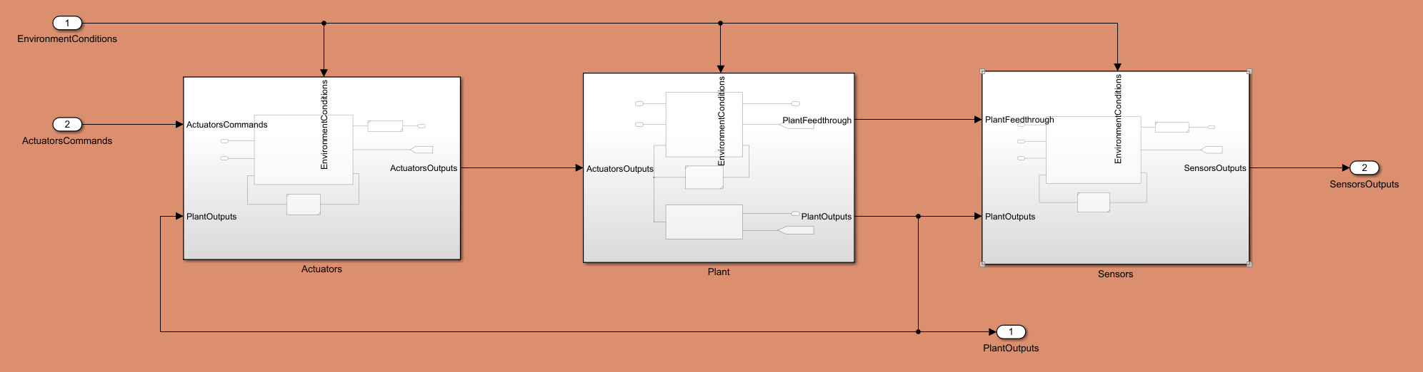
In contrast to the others, the Satellite subsystem is itself just a container for three further subsystems: Plant, Sensors, and Actuators. This is shown in the following picture.

Configuring the Simulink Model

This Simulink model only provides the general structure of the simulation but does not implement any specific functionality. The five main subsystems (Environment, Plant, Sensors, Actuators, GNC Algorithms) contain MATLAB function blocks which in turn call functions defined by files in the UserFiles folder. These are meant to be edited by the user to define the behavior of the simulation. For this, the user can utilize the models provided in the ModelsLibrary folder or implement custom models in the UserFiles folder.

While the naming of the subsystems is meant to provide some guidance on what kind of functionality should be implemented in each, the user is free to decide where to implement what. The only restrictions are the inputs and ouputs of the subsystems. For example, a reaction wheel is an actuator with continuous state dynamics whose functionality the user could implement in the Actuators subsystem. However, if measurements of the wheel speed are needed in the control loop, the user would rather implement the reaction wheel’s state dynamics in the Plant subsystem since only its outputs are directly connected to the Sensors subsystem.

Besides through these functions, the Simulink model is configured through a parameter structure which the user needs to setup and which is passed into the model’s workspace at the beginning of the simulation.

The individual steps to configure the simulation are explained in the Simulation Setup section.

Dynamic Systems

Each of the five main subsystems can be configured by the user to represent a dynamic system with states of their own. For that, each of these subsystems contains a MATLAB function block which is meant to implement both the differential/difference equations of the states update and the algebraic output equation of the system (for background information see Modelling of Dynamic Systems). This way, the user only needs to edit a single MATLAB function for each of these subsystems to define the behavior of the system.

The exception to this is the Plant subsystem which does not only contain one MATLAB function block but two for separating the proper and improper outputs of the system. This prevents Simulink from falsely detecting algebraic loops in the model (as explained in Modelling of Dynamic Systems) because only the proper output PlantOutputs is used in the environment loop.

This is not the case for the control loop since some designs might rely on the usage of improper outputs. E.g., if the plant models the point-mass equations of motion of the satellite, then the inputs to the Plant model would have to directly relate to the satellite’s acceleration. If one wanted to use a measurement of this acceleration within the control loop, it would have to be output by the Plant subsystem. Since it directly depends on the input, it cannot be a proper output. For this reason, the model provides the improper output PlantFeedthrough which is only fed to the Sensors subsystem and is thus only used within the control loop. Usage of this output is optional and can be enabled or disabled by the user through the parameter structure. To prevent an algebraic loop within the control loop, the user is forced to configure a delay somewhere in the subsystems Sensors, GNC Algorithms, or Actuators if the improper output is enabled.

Continuous / Discrete

Through the parameter structure, the user can choose whether the subsystems Sensors, Actuators, and GNC Algorithms should be simulated continuously or with a discrete sample time (Environment and Plant are always continuous). While choosing a discrete sample time for these subsystems might be most realistic, it limits the maximum step size of the simulation. If the systems are configured to be simulated continuously, the Simulink engine can choose the step size freely depending on the system’s dynamics which could speed up the simulation significantly at the cost ignoring the discrete nature of the systems.

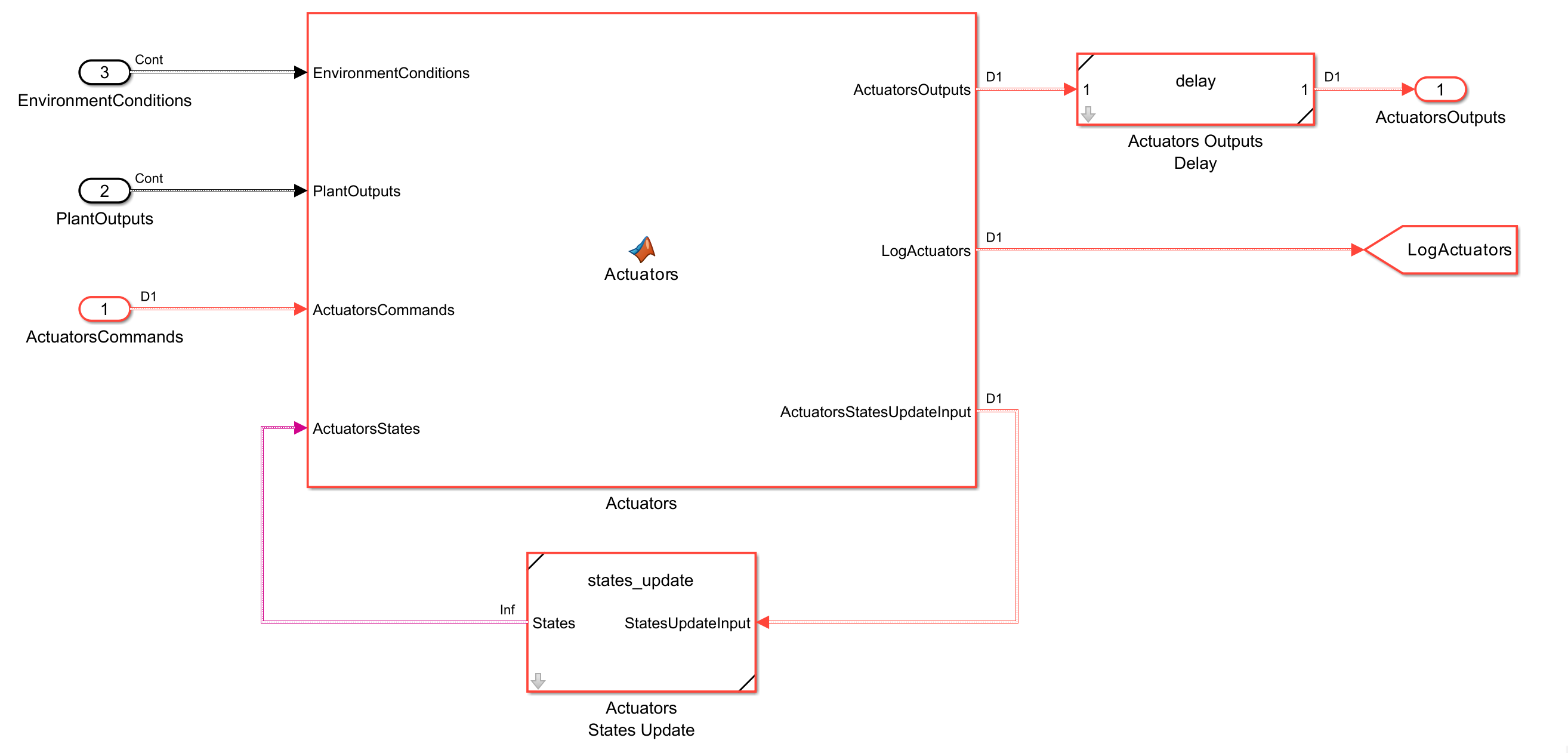
The states update of continuous systems is described by differential equations with respect to time, while the states update of discrete systems is described by difference equations. Therefore, the states update that the Simulink engine performs must be switched between using an integrator for continuous subsystems and a delay for discrete subsystems. This is done automatically depending on the user’s choice by using the utility Simulink model states_update.slx which is included in the Utilities folder. It can be seen below the MATLAB function block in the following picture of the Actuatprs subsystem.

Delays

The user can configure delays for the outputs of the subsystems Sensors, Actuators, and GNC Algorithms to simulate the time it takes for the signals to be processed and passed onto the next subsystem. Depending on whether the subsystem was configured to be simulated continuously or with a discrete sample time, the delay must be implemented either with a continuous Transport Delay block or a discrete Delay block. Similarly to the states update, this is done automatically based on the user’s parametrization by using the utility Simulink model delay.slx which is included in the Utilities folder as well. The block is shown in the above picture before the output port ActuatorsOutputs. As was mentioned in Dynamic Systems, if the user wants to use the improper output PlantFeedthrough, he is forced to configure at least one delay to prevent algebraic loops within the control loop.

Logging

Each MATLAB function block within the five main subsystems has an output port for logging purposes. It is fed into a goto block which directs the signals into the Periphery subsystem on the top level. Here, these signals are marked to be logged. Apart from them, nothing else is logged by the model. So, the user is fully responsible for filling the log signals within the functions called inside the MATLAB function blocks.

docs

The docs folder contains markdown files that are used to generate this documentation website of SADYCOS. Being markdown files, they are already somewhat human-readable when viewed in a text editor and thus can serve as a reference even when there is no access to this documentation website. The user should not need to edit any files within this folder.

UserFiles

As mentioned before, the simulation is structured in a way that should allow the user to avoid editing the contents of the Core folder including the Simulink model file. Instead, the user should implement everything specific to a certain simulation in the UserFiles folder. This folder is made up of the following subfolders:

• Configurations and
• Models.

Configurations

Within SADYCOS, the term configuration is meant to describe all functionalities and parameters needed to set up and run a simulation. This folder should contain classes that each represent a single simulation (or set of similar simulations) and inherit from the abstract superclass SimulationConfiguration provided in the Utilities folder of Core. Such a class encapsulates all the files necessary to implement the desired behavior of the simulation and to configure the parameters of the Simulink model accordingly. The superclass forces its subclasses to implement two sets of static methods.

The methods

• configureParameters and
• configureBuses

are used to setup the parameter structure and the bus objects of the Simulink model, respectively. The parameter structure output by the first method contains a section with general options for the simulations (e.g. the simulation time, the sample time of discrete systems, the output delay of some systems, …) and sections for the models used within the five main subsystems of the Simulink model.

Preparing the bus objects with the second method is necessary because the functions called within the MATLAB function blocks of the Simulink model generally output a structure. Simulink cannot automatically infer the bus objects of the signals from these structures and thus the user has to provide them manually.

The second set of static methods that the subclasses of SimulationConfiguration have to implement consists of the methods

• environment,
• plantDynamics,
• plantOutput,
• sensors,
• actuators,
• gncAlgorithms,
• sendSimData, and stopCriterion (for the Periphery subsystem)

which are the functions called within the MATLAB function blocks of the simulation’s main Simulink model. This is where the user has to manually implement the calls to the models’ execute methods and prepare the output structures that are passed to the next subsystems.

Keeping all these functions encapsulated in classes like this makes switching to simulating a different system as easy as instantiating a different class. The user also benefits from using classes when implementing multiple different simulations which only differ in a few parameters because each class can inherit from some default configuration and would only need to overwrite the corresponding parameters without having to copy the entire rest of the configuration.

Initially, there is a namespace ExampleMission in the Configurations folder which contains a class DefaultConfiguration that serves as an example for how to structure a configuration class.

Models

While the Core contains a library of models that the user can utilize within the simulation, this folder can be used by the user to implement custom models that are specific to the user’s simulation. Like the models in the ModelsLibrary, these models should be subclasses of the abstract superclass ModelBase provided in the Utilities folder of Core.