Modelling of Dynamic Systems

This page is intended to give some background knowledge of how dynamic systems are modelled and simulated in SADYCOS.

Page Contents

• Terminology
  • Simulation
  • Static System
  • Dynamic System
  • Proper Output
  • Improper Output
• Simulink Modelling
  • Generic Dynamic System
  • Separation of Proper and Improper Outputs

Terminology

The following terms are used throughout this page and are briefly explained here:

Simulation

• determination of a system’s behavior over time
• mathematically, this results in the solution of a set of differential/difference equations

Static System

• system output \(y\) depends only on the current input \(u\)

\[y = h(u)\]

Dynamic System

• system output \(y\) depends on the current state \(x\) (and possibly the current input \(u\))

\[y = h(x,u)\]

• states update depends on the current input \(u\) (and possibly the current state \(x\) itself) → system has memory of input history
• two types:
  • continuous: states update is described by a differential equation with respect to time
  \[\dot{x} = f(x,u)\]
  • discrete: states update is described by a difference equation
  \[x_k = f(x_{k-1},u_{k-1})\]
• a dynamic system thus consists of the two static functions \(f\) and \(h\) and a method to update the states

Proper Output

• system output \(y\) does not directly depend on the current input \(u\)
• a proper output of a dynamic system thus only depends on the current state \(x\)

\[y = h(x)\]

• a proper output does not react immediately to changes in the system input but delayed through the system’s dynamics

Improper Output

• system output \(y\) directly depends on the current input \(u\)
• an improper output reacts immediately to changes in the system input → system has direct feedthrough

Simulink Modelling

Simulink simplifies the simulation of dynamic systems because it already provides implementations for common solvers and numerical integration methods. To simulate a continuous dynamic system in a Simulink model, only the static functions \(f\) and \(h\) need to be implemented, e.g. in a MATLAB function block, and connected to an integrator. The Simulink engine then takes care of the numerical solution of the differential equation by figuring out when to call these functions and integrating the ouputs based on the selected solver.

Generic Dynamic System

The following picture shows a generic implementation of such a dynamic system in Simulink with a single block that implements both \(f\) and \(h\), takes \(u\) and \(x\) as inputs, and outputs \(y\) and \(\dot{x}\). The latter is connected to an integrator block which updates \(x\) over time.

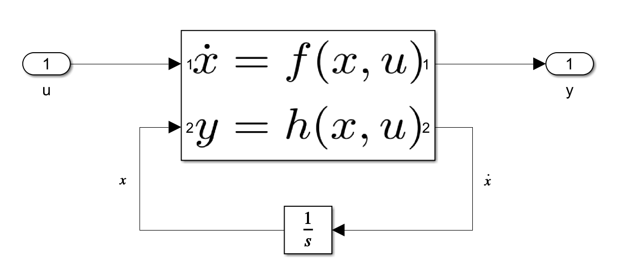
A discrete dynamic system could be implemented in a similar way by outputting the current state instead of its derivative and by replacing the integrator with a delay block.

Many such systems can be chained together by connecting the output of one system to the input of another to create more complex systems. A special kind of such a complex system which is ubiquitous in control engineering is a feedback loop. Here, the output of a system is fed back into its input possibly indirectly through other systems.

Separation of Proper and Improper Outputs

If the output \(y\) depends directly on the input \(u\), it is called an improper output. In a feedback loop, such a chain of improper outputs leads to what is called an algebraic loop within Simulink because the output of the system ends up depending on itself. E.g., if the improper output is fed back directly into the input, one would get the following implicit equation for the output:

\[y = h(x,y).\]

Oftentimes, Simulink can handle these loops with additional numeric solvers at the cost of increased simulation time.

Occasionally, Simulink wrongly concludes that there is an algebraic loop even though there is none. This is the case when \(y\) is actually proper, i.e. the function \(h\) does not depend on \(u\), but \(h\) is implemented in a single MATLAB function block together with \(f\). For those blocks, Simulink does not seem to look into the code itself for finding algebraic loops but rather just relies on the block’s output and input ports. It sees a block that uses \(u\) as an input and outputs \(y\) and cautiously concludes that there might be a direct relation between \(y\) and \(u\). If such a block is part of a feedback loop, Simulink attempts to solve the (non-existent) algebraic loop numerically.

This issue can be avoided altogether by splitting the calculation of proper and improper outputs into separate blocks. The following picture shows such a model where the improper output \(y_1\) is still calculated in the same block as the state derivatives \(\dot{x}\). The proper output \(y_2\), however, is calculated in a separate block that is located behind the integrator and therefore Simulink sees that it only directly depends on the states \(x\) and not the input \(u\).

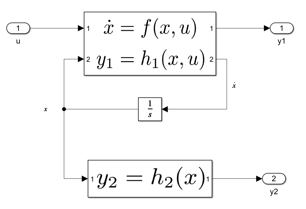
The proper output can then be used in a feedback loop without the risk of Simulink falsely detecting an algebraic loop.